Abaqus Nonlinear Buckling Analysis Methods

Abaqus Nonlinear Buckling Analysis Methods

Abaqus Nonlinear Buckling Analysis Methods

Typically, we only need to ensure that the strength and stiffness of a product structure meet certain requirements or standards. However, in actual engineering, for slender structures or thin-walled structures, we must also consider their stability issues—commonly referred to as instability or collapse problems.

In finite element analysis, we mainly use buckling analysis to determine the critical load at which buckling occurs. Depending on the actual structure and requirements, this is divided into linear buckling analysis (usually simply called buckling analysis) and post-buckling analysis. Of course, if nonlinear issues are involved, post-buckling analysis is necessary. However, implementing post-buckling analysis is more complex, as it requires local adjustments to inp keywords. Nevertheless, mastering the key points makes it manageable through imitation.

In Abaqus, the calculation of buckling depends on the complexity of the structure:

• For simple structures, linear buckling analysis alone can estimate the critical load.
• For more complex models, the Riks method can be used for post-buckling calculations to obtain the structural response after buckling.
• For particularly complex problems involving contact separation, Explicit may be required.
• For local wrinkling issues, Static and Stabilize methods are needed.

01 Linear Buckling Analysis

Linear buckling analysis is used to estimate the critical instability load and instability mode. The calculated buckling eigenvalue multiplied by the applied load gives the critical instability load. Additionally, for buckling problems of perfect structures, linear buckling analysis prepares for introducing defects (disturbances) in post-buckling analysis, which is crucial.

In Abaqus, linear buckling analysis is performed using the Buckle procedure.

Generally, linear buckling analysis only needs to focus on the first-order buckling mode. The first-order buckling load factor is used to estimate the critical load required to cause structural buckling. However, the critical instability load obtained from linear buckling analysis is usually conservative (overestimated). To obtain more accurate results, especially for complex models, nonlinear buckling analysis (or post-buckling analysis) is necessary.

Therefore, keywords are often added in linear buckling analysis as parameters for introducing disturbances in post-buckling analysis. The specific steps are as follows (note the insertion position and format of keywords):

After submitting the calculation, a corresponding .fil file will be generated, which will be referenced in post-buckling analysis!

02 Post-Buckling Analysis

Post-buckling analysis is usually performed after linear buckling analysis. The common approach is to copy the original linear buckling model to create a new model, then adjust and modify analysis steps, load cases, and contact settings. For example, simulating the crushing of a square tube requires changing to explicit dynamic analysis and adding self-contact. Most importantly, defect disturbances must be introduced by calling the previously generated .fil file. The specific steps are as follows:

In the keyword, the name after file refers to the earlier .fil file. The first number "1" in the second line indicates that the disturbance result from the first-order linear buckling is introduced, and "0.5e-3" represents the magnitude of the disturbance.

The size of the disturbance (or defect factor) should ideally be calibrated through experiments. Generally, based on experience, it is set to 0.1% to 0.2% of the shell thickness or rod length.

In practice, you can adjust the disturbance size for trial calculations and compare the post-buckling state with other parameters. If the results change little, the structure is less sensitive to defects; otherwise, it is relatively sensitive. However, this view requires further verification.

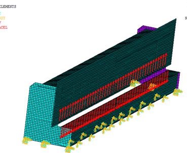
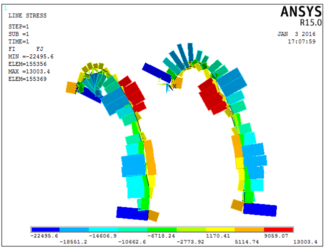
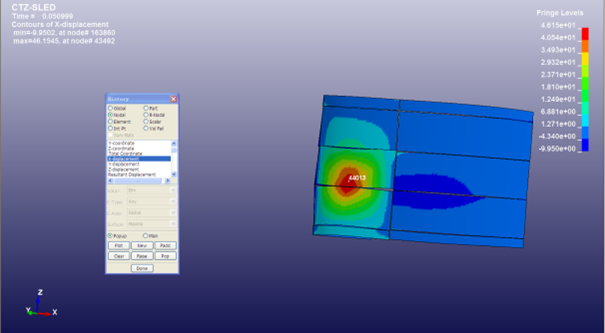
The left figure above shows results without considering disturbances, while the right figure includes disturbances. Observe the differences carefully: the right figure shows a smoother crushing process, making the results more reasonable.

For square tubes, this is actually implemented using the explicit method, which is more accurately called dynamic buckling analysis. Therefore, we must also evaluate energy parameters such as kinetic energy and plastic dissipation to ensure accurate results.

Source: Finite Element Technology Alliance

For details, please contact Teacher Tian: 15029941570