ANSYS Thermal Analysis Example

ANSYS Thermal Analysis Example

ransient Thermal Analysis of a Steel Sphere

Problem Description

Suppose we have a steel sphere with a diameter of 120mm and an initial temperature of 900°C. We need to analyze its temperature change during natural cooling in air, focusing on the temperature distribution within 1 minute.

Analysis Steps

1. Model Establishment: Create the geometric model of the steel sphere in ANSYS Workbench.

2. Material Property Definition: Assign material properties to the steel sphere, including density, specific heat capacity, and thermal conductivity. These properties may vary with temperature.

3. Meshing: Perform meshing on the steel sphere model and select an appropriate mesh size to ensure calculation accuracy.

4. Initial Condition Setup: Set the initial condition, i.e., the initial temperature of the steel sphere is 900°C.

5. Boundary Condition and Load Application:
   Apply a convective heat transfer coefficient on the surface of the steel sphere to simulate the cooling effect of air on the sphere.
   Assume the initial temperature of the surrounding air is 20°C.

6. Solution Type Specification: Select transient thermal analysis, set the total solution time to 60 seconds, and define an appropriate time step.

7. Solution Execution: Run the solver to calculate the temperature field at each time step.

8. Result Post-Processing:
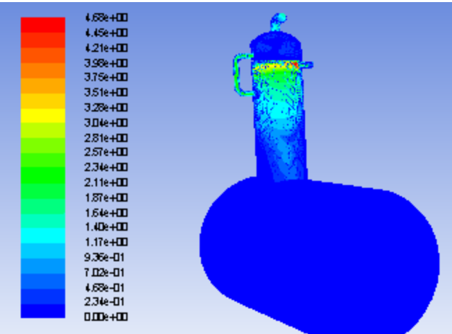
   Extract and observe the temperature distribution contour plots of the steel sphere at different time points.
   Analyze the temperature change trend over time, which can be achieved by setting temperature tracking points at specific locations.

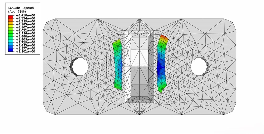
9. Result Evaluation: Evaluate the cooling efficiency of the steel sphere based on the results and determine whether it meets the design requirements.

10. Report Compilation: Prepare an analysis report, including model description, analysis settings, results, and conclusions.

Contact:

Prof. Tian：WhatsApp：+86 15029941570 | Mailbox：540673737@qq.com